Computing Simple Correspondence Analysis
In this section we briefly describe how to compute simple correspondence analysis using CAR (i.e., as a stand-alone application), and car.m (i.e., as a Matlab script). First we present a simple dataset (that can be downloaded from the free-download area of our web site). Then we explain how to load data from files. Finally, we explain how to compute simple correspondence analysis.
Dataset analysed in this tutorial
This example consists of artificial data on the smoking habits of different types of workers in a company (Greenacre 1984, p. 55). Smoking habits were None, Light, Medium, and Heavy; while the types of workers were Senior Managers, Junior Managers, Senior Employees, Junior Employees, and Secretaries.
CAR can read data from text files and from Matlab files (i.e., the typical .mat data files). To replicate our analysis, you should download the file smoke_x.dat. This is a text file that contains two columns of data. The first column is for the variable type of workers, and the second for the variable smoking habit. Figure 1 shows an extract of the information contained in the file.
Figure 1. Short extract of data contained in file smoke_x.dat
	     1     1
	     1     1
	     1     1
	     1     1
	     1     2
	     1     2
	     1     3
	     1     3
    etc
As can be observed in the figure, numerical values must be used to code the information for each individual. The data must also be separated using a white space. In this file, the information is raw data (i.e., individuals’ scores on each variable).
Please note that there will sometimes be a contingency table (instead of the raw data as presented in this file). If this is the case, you can save the contingency table in a text file, and load it to CAR to compute the correspondence analysis from this matrix. If you prefer this option, you can download the data file smoke_Contingence_table.dat.
Figure 2. Labels contained in file smoke_labels_for_rows.txt
	Senior-Managers
	Junior-Managers
	Senior-Employees
	Junior-Employees
	Secretaries
Each label must be a single word, and separations are not allowed. Please note that Matlab users can use more complex labels with more complex Matlab variables (see for example, http://es.mathworks.com/help/matlab/ref/strings.html).
The text file smoke_labels_for_columns.txt contains the labels for the second variable (see figure 3).Figure 3. Labels contained in file smoke_labels_for_columns.txt
	None
	Light
	Medium
	Heavy
Again, each label must be a single word, and separations are not allowed.
To load data from files
Data can be loaded from text files, but also from Matlab data files. The next video shows how to load the three text files presented in the section above.
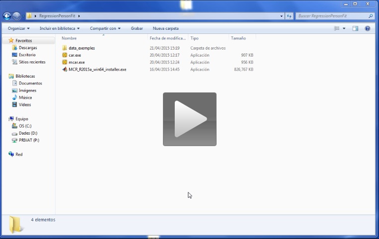
As you can see in the video, the information in each data file is loaded as a variable that must be given a particular name. The name of each variable should be short, comprehensible, and have no special characters (like the addition symbol ‘+’). Once all the variables have been loaded, we advise you to save the information in a Matlab data file: this data file can be loaded in the future if the data need to be reanalysed. The last steps in the video show you how to save data in this way, and how to load it.
Matlab users can load any Matlab file (*.mat), the all the variables in the file will be available in CAR.
How to compute simple correspondence analysis
The next video shows how to compute simple correspondence analysis.
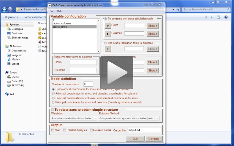
We are analysing raw data stored in X. As X is a matrix with two columns (one column for each variable), we must indicate which column of X is to be placed in the rows of the contingency table, and which column of X is to be placed in the columns. This is the first step in the video. You can use the button Show it to check that you have correctly selected the variables.
The next step is to select the labels for the rows and the columns of the contingency table. Again, you can use the button “Show it” to check that you have correctly selected the labels. CAR will refuse to analyse the data if the number of labels are not consistent with the number of rows and columns of the contingency table. If you do not provide labels, CAR will simply use the numerical values. Figure 4 shows the contingency table for the smoking example.Figure 4. Contingence table related to smoke example
  The 5 x 4 crosstabulation table

Labels             None  Light Medium  Heavy

Senior-Managers       4      2      3      2
Junior-Managers       4      3      7      4
Senior-Employees     25     10     12      4
Junior-Employees     18     24     33     13
Secretaries          10      6      7      2
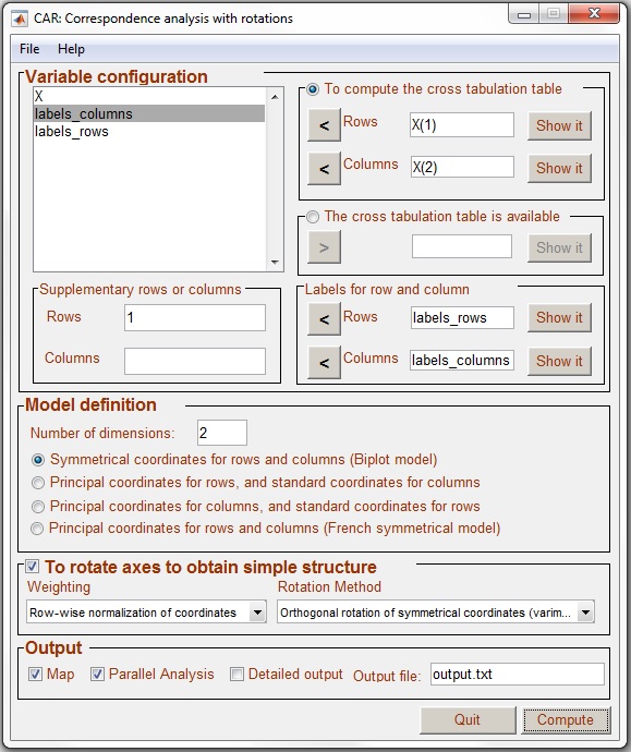
The next step in the analysis is to define (if necessary) the rows or the columns in the contingency matrix that are to be considered as supplementary points in the analysis. For illustrative purposes, we decided to consider senior managers as supplementary points. As this value is the first row of the contingency table, we entered value 1 into the window Rows in the Supplementary rows and columns section. More than one row or column can be indicated just by typing the corresponding number of rows or columns separated with a coma.
The model was defined as: 2 dimensions; and Symmetrical coordinates for rows and columns (Biplot model). We decided to rotate the coordinates using Row-wise normalization of coordinates, and Varimax rotation.
Finally, in the Output, we decided to show the MAP graphical representation of coordinates, compute Parallel Analysis to assess dimensionality, and name the output file output.txt.
Figure 5. CAR configured to analyse smoke data.
Once the analysis has finished, you will find the file output.txt in your working folder as a text file. In addition, the output file is shown using the Windows application Notepad.