Computing Multiple Correspondence Analysis
In this section we briefly describe how multiple correspondence analysis can be computed using MultipleCar (i.e., as a stand-alone application), and MultipleCar.m (i.e., as a Matlab script). First we present a simple dataset (that can be downloaded from the free-download area of our web site). Then we explain how to load data from files. Finally, we explain how to compute multiple correspondence analysis.
Dataset analysed in this tutorial
This example studies the rate of foodborne illness caused by the consumption of vegetables and fruit in the European Union and the United States (Callejón, Rodríguez-Naranjo, Ubeda, Hornedo-Ortega, Garcia-Parrilla & Troncoso, 2015). The illnesses in the analysis were Norovirus, Salmonella spp, Escherichia coli, Campylobacter spp, Shigella spp, Clostridium spp, Staphylococcus spp, Yersinia spp, Bacillus spp, Other viruses, and Other microorganisms. The vegetables were Salad (all produce items related to salad), Leafy (all produce related to leaves, Tomato, and Other vegetables. The fruits were Sprouts (all produce related to sprouts), Berries, Melon, Juices, and Other fruits. For a detailed explanation of the variables, see Table 1 in Callejón et al, 2015.
MultipleCar can read data from text files and from Matlab files (i.e., the typical .mat data files). To replicate our analysis, you should download the file vegetables.dat. This is a text file that contains three columns of data. The first column is the variable illness, the second is the variable vegetables/fruits. And, finally, the third column is the variable region. Figure 6 shows an extract of the information contained in the file.
     …     …     …
     4     3     2
     4     7     2
     4     9     2
     5     1     2
     5     2     2
     5     2     2
     7     1     2
     7     1     2
     9     1     2
     9     9     2
    10     2     2
	etc
As can be observed in the figure, numerical values must be used to code the information for each observation. The data must also be separated using a white space. In this file, the information is the raw data.
Please note that sometimes there will be an Indicator matrix or a Burt Contingency table (instead of the raw data presented in this file). If this is the case, you can save your indicator matrix or your Burt contingency table in a text file, and load it to MultipleCar to compute multiple correspondence analysis of these matrices.
In order for the output of the analysis to be more interpretable, the numerical codification of data can be labelled. The text file vegetables_labels.txt contains the labels for the three variables (see figure 7).
Figure 7. Labels contained in file vegetables_labels.txt
  Norovirus
	Salmonella
	E-coli
	Campylobacter
	Shigella
	Clostridium
	Staphylococcus
	Yersinia
	Bacillus
	Other-viruses
	Other-microorganisms
	Salad
	Leafy
	Tomato
	Other-vegetables
	Sprouts
	Berries
	Melon
	Juices
	Other-fruits
	EU
	USA
Each label must be a single word, and separations are not allowed. Please note that Matlab users can use more complex labels with more complex Matlab variables (see for example, http://es.mathworks.com/help/matlab/ref/strings.html). In addition, please note that the labels for the three variables (illness, vegetable/fruit and region) must be in the same order as in the columns in the raw data (the same applies when analysing Indicator or Burt contingency matrices).
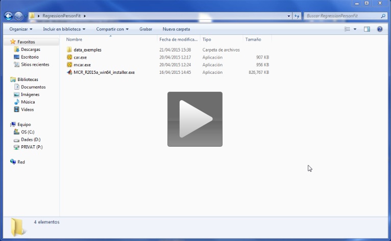
To load data from files
Data can be loaded from text files, but also from Matlab data files. The next video shows how to load the three text files presented in the section above.
As you can see in the video, the information in each data file is loaded as a variable that must be given a particular name. The name of each variable should be short, comprehensible, and have no special characters (like the addition symbol ‘+’). Once all the variables have been loaded, we advise you to save the information in a Matlab data file: this data file can be loaded in the future if the data need to be reanalysed. The last steps in the video show you how to save data in this way, and how to load it.
Matlab users can load any Matlab file (*.mat), the all the variables in the file will be available in MultipleCar.
How to compute multiple correspondence analysis
The next video shows how to compute multiple correspondence analysis.
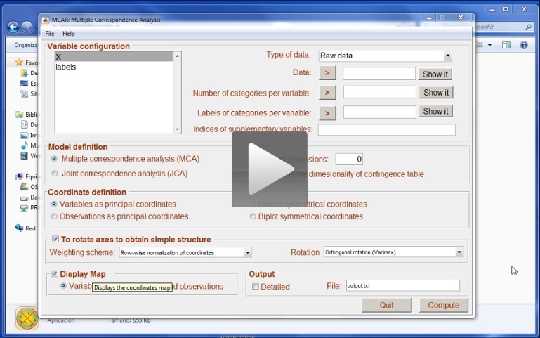
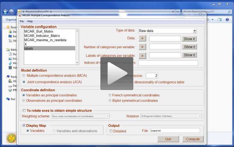
We are analysing raw data stored in X. As X is a matrix that contains raw data, we have the label Raw data in the drop-box. This is the first step in the video. You can use the button “Show it” to check that you have correctly selected the variable.
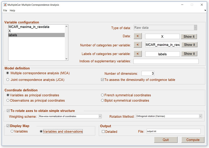
After selecting a matrix as a Raw data matrix, MultipleCar computes a new variable: MCAR_maxima_in_rawdata. If the variables in X have been coded using consecutive numbers starting from 1, this new variable properly defines the number of categories in each of the three raw variables. This variable needs to be selected in the window Number of categories per variable. After selecting this variable, you can check if MultipleCar has correctly computed the number of categories in your variables using the button Show it. If you observe that the number of categories in MCAR_maxima_in_rawdata is wrong, then you should store the correct values in a text file, and load them as a variable.
The next step is to select the labels. Again, you can use the button Show it to check that you have correctly selected the labels. MultipleCar will refuse to analyse the data if the number of labels are not consistent with the number of variables and categories per variable. If you do not provide labels, MultipleCar will simply use the numerical values.
The next step in the analysis is to define (if necessary) the variables that are to be considered as supplementary points in the analysis. For illustrative purposes, we decided to consider regions as supplementary points. As this is the third variable in the raw data, we entered value 3 into the window Indices in the Supplementary variables section. More than one variable can be indicated just by typing the corresponding number of variable separated with a coma.
The model was defined selecting the following options in the main menu: Multiple correspondence analysis with 2 dimensions; To assess the dimensionality of the contingency table, and Variables as principal coordinates. We decided to rotate the coordinates using Row-wise normalization of coordinates, and Varimax rotation.
Finally, in the Output, we decided to show the MAP graphical representation of coordinates, and name the output file output.txt.
Figure 8. MultipleCar configured to analyse vegetable data.
Once the analysis has finished, you will find the file output.txt in your working folder as a text file. In addition, the output file is shown using the Windows application notepad. The figure can be manipulated to help to display the configuration. Matlab users may have more options in this manipulation.
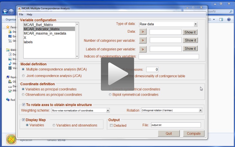
Once the analysis has finished, users will realise that two variables are available: MCAR_Indicator_Matrix and MCAR_Burt_Matrix. These two matrices can be analysed in the future so we suggest that you save the data. Computing the Indicator matrix is a time consuming process: if the matrix has already been computed, new analysis of the same data can be much faster. The next video shows how to compute multiple correspondence analysis from the Indicator matrix. Note that the first analysis using the raw matrix was done in 0.685 seconds, while the second (using the Indicator matrix) was done in 0.23 seconds. With large datasets, the difference could turn out to be quite significant.
The next video shows how to compute multiple correspondence analysis from the Burt matrix: in this case we opted for a Joint Correspondence analysis. Please note that the number of options available when computing multiple correspondence analysis from the Burt matrix are limited.
References
Callejón, R. M., Rodríguez-Naranjo, M. I., Ubeda, C., Hornedo-Ortega, R., Garcia-Parrilla, M. C., & Troncoso, A. M. (2015). Reported Foodborne Outbreaks Due to Fresh Produce in the United States and European Union: Trends and Causes. Foodborne pathogens and disease, 12(1), 32-38.